Introduction ¶

Contents

Introduction

Introduction ¶

This is a brief introduction to skrf which highlights a range of features without going into detail on any single one. At the end of each section there are links to other tutorials, that provide more information about a given feature. The intended audience are those who have a working python stack, and are somewhat familiar with python. If you are unfamiliar with python, please see scipy’s Getting Started .

Although not essential, these tutorials are most easily followed by using the ipython shell with the --pylab flag.

> ipython --pylab
In [1]:

Using ipython with the pylab flag imports several commonly used functions, and turns on interactive plotting mode which causes plots to display immediately.

Throughout this tutorial, and the rest of the scikit-rf documentation, it is assumed that skrf has been imported as rf. Whether or not you follow this convention in your own code is up to you.

In [1]: import skrf as rf

If this produces an error, please see Installation.

Note

The example code in these tutorials make use of files that are distributed with the source package. The working directory for these code snippets is scikit-rf/doc/, hence all data files are referenced relative to that directory. If you do not have the source package, then you may access these files through the skrf.data module (ie from skrf.data import ring_slot)

Networks ¶

The Network object represents a N-port microwave Network. A Network can be created in a number of ways. One way is from data stored in a touchstone file.

In [1]: ring_slot = rf.Network('../skrf/data/ring slot.s2p')

A short description of the network will be printed out if entered onto the command line

In [1]: ring_slot
Out[1]: 2-Port Network: 'ring slot',  75-110 GHz, 201 pts, z0=[ 50.+0.j  50.+0.j]

he basic attributes of a microwave Network are provided by the following properties :

Network.s : Scattering Parameter matrix.
Network.z0 : Port Characterisic Impedance matrix.
Network.frequency : Frequency Object.

All of the network parameters are complex numpy.ndarray ‘s of shape FxNxN, where F is the number of frequency points and N is the number of ports. The Network object has numerous other properties and methods which can found in the Network docstring. If you are using IPython, then these properties and methods can be ‘tabbed’ out on the command line.

In [1]: short.s<TAB>
rf.data.line.s              rf.data.line.s_arcl         rf.data.line.s_im
rf.data.line.s11            rf.data.line.s_arcl_unwrap  rf.data.line.s_mag
...

Linear Operations ¶

Element-wise mathematical operations on the scattering parameter matrices are accessible through overloaded operators. To illustrate their usage, load a couple Networks stored in the data module.

In [1]: short = rf.data.wr2p2_short

In [2]: delayshort = rf.data.wr2p2_delayshort

In [3]: short - delayshort
Out[3]: 1-Port Network: 'wr2p2,short',  330-500 GHz, 201 pts, z0=[ 50.+0.j]

In [4]: short + delayshort
Out[4]: 1-Port Network: 'wr2p2,short',  330-500 GHz, 201 pts, z0=[ 50.+0.j]

Cascading and De-embedding ¶

Cascading and de-embeding 2-port Networks can also be done though operators. The cascade() function can be called through the power operator, **. To calculate a new network which is the cascaded connection of the two individual Networks line and short,

In [1]: short = rf.data.wr2p2_short

In [2]: line = rf.data.wr2p2_line

In [3]: delayshort = line ** short

De-embedding can be accomplished by cascading the inverse of a network. The inverse of a network is accessed through the property Network.inv. To de-embed the short from delay_short,

In [1]: short = line.inv ** delayshort

For more information on the functionality provided by the Network object, such as interpolation, stitching, n-port connections, and IO support see the Networks tutorial.

Plotting ¶

Amongst other things, the methods of the Network class provide convenient ways to plot components of the network parameters,

Network.plot_s_db() : plot magnitude of s-parameters in log scale
Network.plot_s_deg() : plot phase of s-parameters in degrees
Network.plot_s_smith() : plot complex s-parameters on Smith Chart
...

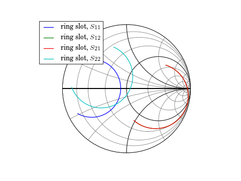
To plot all four s-parameters of the ring_slot on the Smith Chart.

In [1]: ring_slot.plot_s_smith();

For more detailed information about plotting see the Plotting tutorial

NetworkSet ¶

The NetworkSet object represents an unordered set of networks and provides methods for calculating statistical quantities and displaying uncertainty bounds.

A NetworkSet is created from a list or dict of Network‘s. This can be done quickly with read_all() , which loads all skrf-readable objects in a directory. The argument contains is used to load only files which match a given substring.

In [1]: rf.read_all('../skrf/data/', contains='ro')
Out[1]: 
{'ro,1': 1-Port Network: 'ro,1',  500-750 GHz, 201 pts, z0=[ 50.+0.j],
 'ro,2': 1-Port Network: 'ro,2',  500-750 GHz, 201 pts, z0=[ 50.+0.j],
 'ro,3': 1-Port Network: 'ro,3',  500-750 GHz, 201 pts, z0=[ 50.+0.j]}

This can be passed directly to the NetworkSet constructor,

In [1]: ro_dict = rf.read_all('../skrf/data/', contains='ro')

In [2]: ro_ns = rf.NetworkSet(ro_dict, name='ro set') #name is optional

In [3]: ro_ns
Out[3]: A NetworkSet of length 3

Statistical Properties ¶

Statistical quantities can be calculated by accessing properties of the NetworkSet. For example, to calculate the complex average of the set, access the mean_s property

In [1]: ro_ns.mean_s
Out[1]: 1-Port Network: 'ro set',  500-750 GHz, 201 pts, z0=[ 50.+0.j]

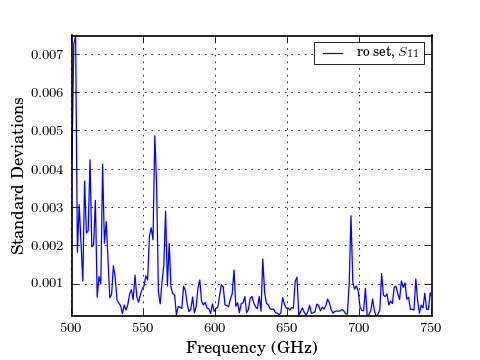
Similarly, to calculate the complex standard deviation of the set,

In [1]: ro_ns.std_s
Out[1]: 1-Port Network: 'ro set',  500-750 GHz, 201 pts, z0=[ 50.+0.j]

These methods return a Network object, so the results can be saved or plotted in the same way as you would with a Network. To plot the magnitude of the standard deviation of the set,

In [1]: figure();

In [2]: ro_ns.std_s.plot_s_re(y_label='Standard Deviations')

Plotting Uncertainty Bounds ¶

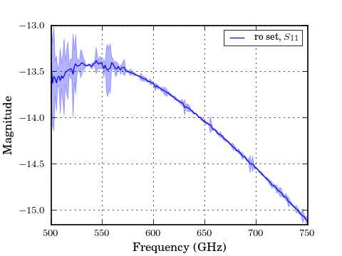
Uncertainty bounds on any network parameter can be plotted through the methods

In [1]: figure();

In [2]: ro_ns.plot_uncertainty_bounds_s_db()

../_images/ns_plot_uncertainty_bounds_s_db.png

See the NetworkSet tutorial for more information.

Virtual Instruments ¶

Warning

The vi module is not well written or tested at this point.

The vi module holds classes for GPIB/VISA instruments that are intricately related to skrf, mostly VNA’s. The VNA classes were created for the sole purpose of retrieving data so that calibration and measurements could be carried out offline by skrf, control of most other VNA capabilities is neglected.

Note

To use the virtual instrument classes you must have pyvisa installed.

A list of VNA’s that have been are partially supported.

An example usage of the HP8510C class to retrieve some s-parameter data

In [1]: from skrf.vi import vna

In [2]: my_vna = vna.HP8510C(address =16)

#if an error is thrown at this point there is most likely a problem with your visa setup
In [3]: dut_1 = my_vna.s11

In [4]: dut_2 = my_vna.s21

In [5]: dut_3 = my_vna.two_port

Unfortunately, the syntax is different for every VNA class, so the above example wont directly translate to other VNA’s. Re-writing all of the VNA classes to follow the same convention is on the TODO list

See the virtualInstruments tutorial for more information.

Calibration ¶

skrf has support for one and two-port calibration. skrf‘sdefault calibration algorithms are generic in that they will work with any set of standards. If you supply more calibration standards than is needed, skrf will implement a simple least-squares solution. skrf does not currently support TRL.

Calibrations are performed through a Calibration class. Creating a Calibration object requires at least two pieces of information:

a list of measured Network‘s
a list of ideal Network‘s

The Network elements in each list must all be similar (same #ports, frequency info, etc) and must be aligned to each other, meaning the first element of ideals list must correspond to the first element of measured list.

Optionally, other information can be provided when relevent such as,

calibration algorithm
enforce eciprocity of embedding networks
etc

When this information is not provided skrf will determine it through inspection, or use a default value.

Below is an example script illustrating how to create a Calibration . See the Calibration tutorial for more details and examples.

One Port Calibration ¶

This example is the same as the first except more concise.

import skrf as rf

my_ideals = rf.read_all('ideals/')
my_measured = rf.read_all('measured/')
duts = rf.read_all('measured/')

## create a Calibration instance
cal = rf.Calibration(\
        ideals = [my_ideals[k] for k in ['short','open','load']],
        measured = [my_measured[k] for k in ['short','open','load']],
        )

caled_duts = [cal.apply_cal(dut) for dut in duts.values()]

Media ¶

skrf supports the microwave network synthesis based on transmission line models. Network creation is accomplished through methods of the Media class, which represents a transmission line object for a given medium. Once constructed, a Media object contains the neccesary properties such as propagation constant and characteristic impedance, that are needed to generate microwave circuits.

The basic usage looks something like this,

In [1]: import skrf as rf

In [2]: freq = rf.Frequency(75,110,101,'ghz')

In [3]: cpw = rf.media.CPW(freq, w=10e-6, s=5e-6, ep_r=10.6)

In [4]: cpw.line(100*1e-6, name = '100um line')
Out[4]: 2-Port Network: '100um line',  75-110 GHz, 101 pts, z0=[ 50.06074662+0.j  50.06074662+0.j]

Warning

The network creation and connection syntax of skrf are cumbersome if you need to doing complex circuit design. For a this type of application, you may be interested in using QUCS instead. skrf‘s synthesis cabilities lend themselves more to scripted applications such as Design Optimization or batch processing.

Media Types ¶

Specific instances of Media objects can be created from relevant physical and electrical properties. Below is a list of mediums types supported by skrf,

Network Compoents ¶

Here is a brief list of some generic network components skrf supports,

Usage of these methods can is demonstrated below.

To create a 1-port network for a coplanar waveguide short (this neglects dicontinuity effects),

In [1]: cpw.short(name = 'short')
Out[1]: 1-Port Network: 'short',  75-110 GHz, 101 pts, z0=[ 50.06074662+0.j]

Or to create a $90^{\circ}$ section of cpw line,

In [1]: cpw.line(d=90,unit='deg', name='line')
Out[1]: 2-Port Network: 'line',  75-110 GHz, 101 pts, z0=[ 50.06074662+0.j  50.06074662+0.j]

See Media for more information about the Media object and network creation.

Introduction ¶

Introduction ¶

Networks ¶

Linear Operations ¶

Cascading and De-embedding ¶

Plotting ¶

NetworkSet ¶

Statistical Properties ¶

Plotting Uncertainty Bounds ¶

Virtual Instruments ¶

Calibration ¶

One Port Calibration ¶

Media ¶

Media Types ¶

Network Compoents ¶

Table Of Contents

Previous topic

Next topic

This Page

Navigation

Previous topic

Next topic

This Page

Quick search

Navigation